Contact Us
Subscribe to Causeway Insights, delivered to your inbox.
In the past two years, value stocks, along with cyclicals and higher-volatility equities, have underperformed broader markets while higher-momentum stocks have outperformed. When will these trends change? Here, we use a quantitative approach to examine these style factors relative to history from three different perspectives.
First, we observe that the current valuation dispersion in these factors (e.g., the discount of value stocks relative to their expensive peers, and the premium attached to high-momentum stocks) is much greater than historical averages, creating a potentially heightened probability for mean reversion. Next, we find that the current spreads in valuation multiples are not explained by spreads in earnings growth and returns on equity (ROE) expectations - the key drivers of price-to-earnings (P/E) and price-to-book value (P/B) ratios. Finally, by examining past drawdowns in value and momentum factors, the analysis indicates that when the mean reversion comes, the “snap-back” will likely happen quickly.
Value investing has always been an inherently unpopular and lonely road to travel. Cheap stocks tend to trade at discounts to peers for a reason, though the academic debate continues as to whether that reason is more risk-based or behavioral in nature. Risk-based proponents argue that value stocks price in a higher probability of financial distress. More generally, those stocks may reflect greater perceived uncertainty around future earnings created from cyclical, structural, or competitive forces. Behavioral explanations focus instead on the practical limitations facing market participants. Many investors simply do not have the mandate, liquidity, patience, or conviction to maintain these unpopular positions for extended periods of time. Value stocks can take years to “re-rate” upward, and holding these out-of-favor stocks will likely cause short-term pain. As with any consistent investing strategy, a value style will underperform the broader market from time to time. This is simply the price of being contrarian.
Value investing has always been an inherently unpopular and lonely road to travel.
So why invest in value at all? Its track record is perhaps value’s strongest advocate. Over longer periods, value stocks have outperformed the markets fairly consistently. As Exhibit 1 illustrates, despite short periods of weakness, value indices have outperformed benchmark indices over the past 25 years. Additionally, buying inexpensive or “cheap,” unloved stocks makes intuitive sense. If a stock trades lower but fundamentals remain unchanged, the upside to downside ratio improves and the increasingly asymmetric return profile becomes more attractive. At Causeway, we like to add to positions on these price declines. It may be difficult to do at the time, but this discipline is why you hire an active value manager. Although timing cannot be predicted, eventually value works, the pendulum swings the other way, and cheap stocks ultimately outperform. Contrarian investors who can “stomach” value drawdowns are rewarded for their patience by the subsequent snap-back and re-rating.
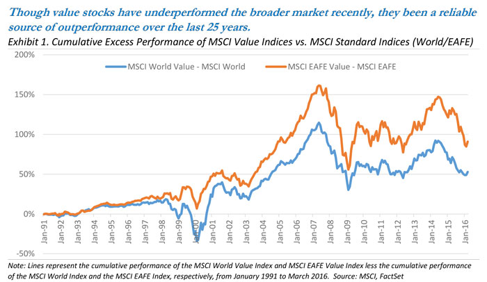
Despite a small bounce in March 2016, however, value stocks have underperformed broader market indices since the summer of 2014. The questions that follow are, how long can this underperformance persist, and at what point might value resume its historical leadership? While identifying the precise turning point is not possible, we can search for indications by examining past valuation spreads, disconnects between market multiples and their respective drivers, and the structure of previous drawdowns. Though our primary style factor focus is value, we also analyze momentum, cyclicality, and volatility* given recent trends.
*“Value” measures a stock’s relative cheapness, “momentum” measures a stock’s relative price performance, “cyclicality” measures a stock’s sensitivity to economic cycles, and “volatility” measures a stock’s historical variability.
I. Dispersion in the Valuation Ratios of Style Factors is Elevated Relative to History
We begin by measuring how cheaply or expensively each of these four styles is trading relative to the last 25 years. We use 25 years based on the availability of constituent-level data for the MSCI World Index. At the end of each month, we distribute the constituents of the MSCI World Index into quintiles based on each stock’s relative exposure to a specific style. For each factor, we use Causeway’s risk model definitions which combine multiple measures of each style exposure. Next, we observe the median price-to-book value and forward price-to-earnings multiple for those stocks sorted into the extreme quintiles (the top quintile, or “Q1” and the bottom quintile, or “Q5”). Finally, we track the ratio of the median valuation multiple of Q1 relative to the median valuation multiple of Q5. Comparing the most recent measure of this dispersion ratio to its range over the past 25 years will give us a sense of how far away the current ratio is from norms over the period.
Exhibit 2 plots the most recent data point for each style factor standardized relative to its 25-year history. Current points are plotted in terms of standard deviations from the 25-year median (to diminish the impact of historical outliers). If a particular factor’s dispersion is either well above or well below its 25-year norm, we would argue that it is overvalued or undervalued, respectively. The gray bars reference a +/- 1 standard deviation difference from the median of the respective valuation ratio between extreme quintiles.
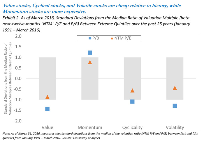
We see from Exhibit 2 that the valuation ratio of cheap stocks relative to expensive stocks is roughly a 1 standard deviation discount to 25-year historical norms on a P/E basis and even greater on a P/B basis. Stated differently, cheap stocks usually do not trade so cheaply, and value as a factor appears oversold. Momentum exhibits the opposite characteristic. High momentum stocks are trading at a much larger premium to low momentum stocks relative to their 25-year history. Additionally, we observe that cyclical stocks are trading at a larger discount to less cyclical (or “defensive”) stocks compared to their 25-year history, and higher-volatility stocks are also trading at a greater discount to lower-volatility stocks. These findings are consistent with recent relative performance: Value has underperformed, while momentum, defensive, and “low-vol” stocks all have outperformed.
Why do we care about the current valuation dispersion of each style factor relative to history? All of these factors have a tendency toward mean reversion. And we believe Causeway value equity strategies are well-positioned for such a turn. In our international and global value portfolios, we currently have positive active exposure (exposure relative to that of the benchmark index) to value and cyclicality, and we have negative active exposure to momentum. Mean reversion in these factors should benefit Causeway portfolios. It is important to emphasize that these active positions do not represent attempts to “time” factors. Rather, as value investors, we will generally have positive active exposure to undervalued factors and negative active exposure to overvalued factors.
II. Spreads in Fundamental Drivers Do Not Explain Differences in Current Valuation Multiples
Another way to gauge the degree of disconnect in factor valuations is to investigate the drivers behind the specific metrics that we have been using: price-to-earnings and price-to-book value multiples. Using the Gordon Growth Model framework, we know that a stock price (P) should reflect the growing stream of future earnings per share (Et+1 growing by g), assuming all earnings are paid as dividends, discounted by the cost of equity (re):

If the market is efficient, a stock’s price should adjust to equal future earnings per share (EPS) divided by the difference between the cost of equity and the EPS growth rate. Rearranging the terms, the P/E multiple should equal the reciprocal of the difference between the cost of equity and the growth rate. As the equation indicates, investors should be willing to pay a higher P/E multiple for stocks exhibiting higher earnings growth. Although the cost of equity is admittedly an important determinant of a P/E multiple, we find that the relationship between market beta (a key input in CAPM-derived re) and valuation quintile is not stable historically. Expected earnings growth (g), on the other hand, has consistently been positively correlated with P/E, and we will therefore focus on growth differentials in this analysis.
If we reframe the first equation from above in terms of the dividend discount model and relax the assumption of a 100% payout ratio, we are able to see what drives the price-to-book value (BV0 ) multiple:
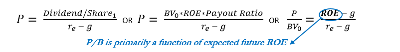
We assume that g = 1 – Payout ratio, so Payout ratio = 1 – g.
Since P/E multiples are driven by expected earnings growth, and P/B multiples are driven by expected future Return on Equity (ROE), we will compare current P/E multiples to growth rates and current P/B multiples to ROEs. Exhibit 3 shows these comparisons for the four style factors that we have been examining. We compare the median P/E multiple of extreme quintiles with the respective median rolling FY3/FY1 growth rate**. We also compare the median P/B multiple with the respective median ROE. With these data, we can observe whether the current inter-quintile spread in growth rates explains the spread in P/E multiples, and whether the current spread in ROE explains the spread in P/B multiples. As the formulas above indicate, these relationships are not linear and our analysis does not mean to suggest that they are, however the drivers nevertheless share a direct relationship to the market multiples.
** We acknowledge that the “g” in the equations above is meant to represent growth in perpetuity, however due to data availability and reliability issues with long-term growth (“LTG”) estimates, we rely on FY3/FY1 EPS growth estimates as a proxy.
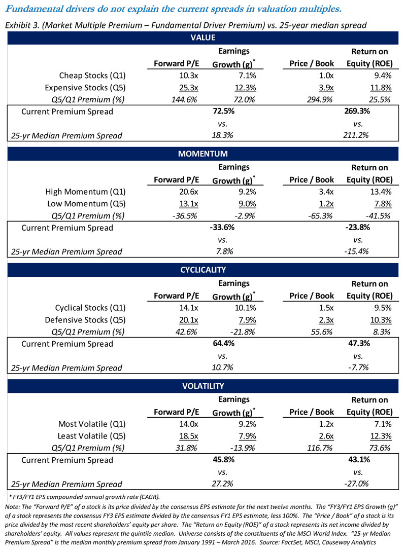
In the cases of value, cyclicality, and volatility, the spread in market multiples far outpaces the spread in the underlying driver. This shows yet again that value stocks, cyclical stocks, and higher-volatility stocks are trading at much bigger discounts to their opposing peers relative to the underlying driver. Admittedly, a valuation premium is probably warranted from more “stable” defensive and low-volatility stocks, but the current valuation spreads are also much greater than their 25-year median spreads (see the boxed comparison). In the case of momentum, high-momentum stocks trade at a much larger premium than the underlying drivers or historical spreads would justify. Again, this is consistent with our conclusions in Exhibit 2.
Value stocks, cyclical stocks, and higher-volatility stocks are trading at much bigger discounts to their opposing peers relative to the underlying driver.
III. Previous Factor Drawdowns
Finally, in the case of value and momentum specifically, it is helpful to examine the characteristics of past drawdowns for insights into mean reversion trends. Using our proprietary risk model, which strips out the effects of individual styles from country, sector, currency, and idiosyncratic effects, we seek to isolate and link the historical returns attributable to value. These would be the theoretical returns that any portfolio with a pure exposure to value (holding all other factors constant) would have recognized. And as such, we believe they offer a good proxy for the effects impacting value portfolios such as Causeway’s international and global value strategies. Exhibit 4 analyzes the characteristics of previous value drawdowns over the past 25 years (1991 – March 2016) using a broad universe of global equities in the developed markets.
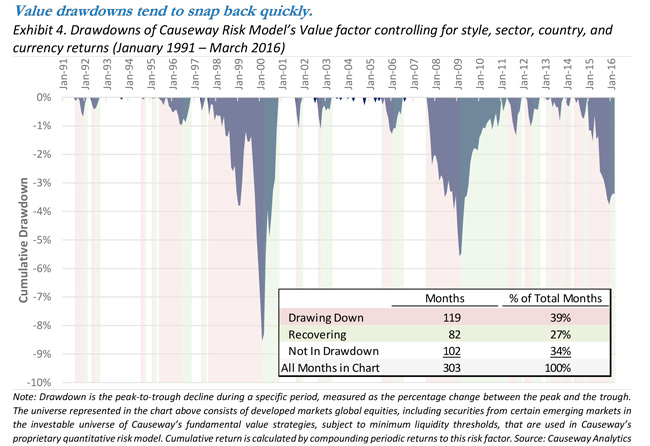
For this analysis, we define a drawdown as any decline lasting two or more months in order to avoid single down months. The average number of months to trough was 6.6 months, and average recovery period was 4.6 months, equating to an average total drawdown period of approximately 11 months. Two observations can be drawn from these statistics. First, we are currently 15 months into a drawdown for value (12 months if the December trough holds), well above the typical trough period of 6.6 months. Second, the average recovery period from a trough is much shorter than the period to the trough. Returns to value tend to recover quickly, which means that attempting to time the bottom may result in a missed recovery. In fact, looking at the table in Exhibit 4, we see that over the past 25+ years, 39% of months were spent drawing down, while only 27% were recovering. This is also consistent with the positive skew in returns to value, indicating that the magnitude of positive returns eclipses the more numerous, smaller declines. Out of the four factors we have discussed, value is the only one with a positive skew (meaning that the other factors experience larger-magnitude negative returns).
Returns to value tend to recover quickly, which means that attempting to time the bottom may result in a missed recovery.
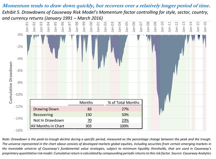
Unlike value, momentum has performed very well recently and as contrarian value managers, we have a negative exposure to momentum. However, it is interesting to note that the drawdown pattern is reversed for momentum. Momentum tends to draw down very quickly to its trough, but recovers over a relatively longer period of time. The typical period to trough is 4.9 months compared to the 8.8 month average recovery. Over the past 25+ years, we have witnessed nearly twice as many months in which momentum was recovering than drawing down. Since our value and momentum factors have a -.24 correlation, it is possible that momentum could experience a drawdown at a similar time that value snaps out of a drawdown (and indeed the past several months have witnessed the beginning of a drawdown for momentum). Both would likely be beneficial for Causeway’s developed equity portfolios.
Summary
The recent underperformance of value as an investment style has created a strong headwind for value managers, prompting the question, when will value resume its historical outperformance? We seek to answer this question by measuring the magnitude of the current dislocation from three perspectives. We find that value stocks are trading at a much larger discount to their more expensive peers relative to history. They are also much more disconnected from their underlying valuation drivers relative to history. And finally, the drawdown in value has already outpaced the average previous decline. Although recovery could still take longer given the depth of the current drawdown, each of these analyses argue in favor of mean reversion for value. We believe the time to emphasize value has arrived.
This paper expresses the portfolio managers’ views as of April 2016 and should not be relied on as research or investment advice regarding any stock. These views and any portfolio holdings and characteristics are subject to change. There is no guarantee that any forecasts made will come to pass.
International investing may involve risk of capital loss from unfavorable fluctuations in currency values, from differences in generally accepted accounting principles, or from economic or political instability in other nations.
The MSCI EAFE Index is a free float adjusted market capitalization weighted index, designed to measure developed market equity performance excluding the U.S. and Canada, consisting of 21 stock markets in Europe, Australasia, and the Far East. The MSCI World Index is a free float-adjusted market capitalization index, designed to measure developed market equity performance, consisting of 23 developed country indices, including the U.S. The MSCI EAFE Value and MSCI World Value Indices are subsets of these indices, and target 50% coverage of the MSCI EAFE Index and MSCI World Index, respectively, with value investment style characteristics for index construction using three variables: book value to price, 12-month forward earnings to price, and dividend yield. The indices are gross of withholding taxes, assume reinvestment of dividends and capital gains, and assume no management, custody, transaction or other expenses. It is not possible to invest directly in an Index.
MSCI has not approved, reviewed or produced this report, makes no express or implied warranties or representations and is not liable whatsoever for any data in the report. You may not redistribute the MSCI data or use it as a basis for other indices or investment products.
“Beta” is a measure of the risk potential of a stock or an investment portfolio expressed as a ratio of the stock’s or portfolio’s volatility to the volatility of the market as a whole.
“CAPM” or the “Capital Asset Pricing Model” provides a formula that calculates the expected return on a security based on its level of risk. The formula for the capital asset pricing model is the risk free rate plus beta times the difference of the return on the market and the risk free rate.
“Gordon Growth Model” is used to determine the intrinsic value of a stock based on a future series of dividends that grow at a constant rate. Given a dividend per share that is payable in one year, and the assumption the dividend grows at a constant rate in perpetuity, the model solves for the present value of the infinite series of future dividends.
“Standard Deviation” is a measure that is used to quantify the amount of variation or dispersion of a set of data values. The more spread apart the data, the higher the deviation. Standard deviation is calculated as the square root of variance.